ResNet, Deep Residual Learning for Image Recognition
Is learning better networks as easy as stacking more layers?
- Original Paper: Deep Residual Learning for Image Recognition
- GitHub Repo: Deep Learning Classics: Read, Review, Recode
Abstract
Deeper neural networks are more difficult to train. We present a residual learning framework to ease the training of networks that are substantially deeper than those used previously. We explicitly reformulate the layers as learning residual functions with reference to the layer inputs, instead of learning unreferenced functions.
We provide comprehensive empirical evidence showing that these residual networks are easier to optimize, and can gain accuracy from considerably increased depth. On the ImageNet dataset, we evaluate residual nets with a depth of up to 152 layer, 8× deeper than VGG nets but still having lower complexity. An ensemble of these residual nets achieves 3.57% error on the ImageNet test set.
This result won the 1st place on the ILSVRC 2015 classification task. We also present analysis on CIFAR-10 with 100 and 1000 layers. The depth of representations is of central importance for many visual recognition tasks. Solely due to our extremely deep representations, we obtain a 28% relative improvement on the COCO object detection dataset. Deep residual nets are the foundations of our submissions to ILSVRC & COCO 2015 competitions, where we also won the 1st places on the tasks of ImageNet detection, ImageNet localization, COCO detection, and COCO segmentation.
Background & Problematic
Well, basically the rule was like: “the deeper the networks, the better.”
Indeed, as you must know, the inner advantage of neural networks (NN) is their natural ability to learn low/mid/high-level features. So in theory, the “levels” of features can be enriched by the number of stacked layers (depth), and over time, many visual recognition tasks have greatly benefited from very deep models.
 ResNet meme
“Is learning better networks as easy as stacking more layers?”
The short answer is NO! They showed empirically that when deeper networks are able to start converging, a degradation problem has been exposed: with the network depth increasing, accuracy gets saturated and then degrades rapidly. In simple words, adding more layers to a suitably deep model leads to higher training and test error.
This result is counterintuitive as a deeper model can theoretically match or even outperform a shallower one by copying its parameters and adding identity layers, but in practice, it’s not the case.
Core Idea: Residual Learning
The deep residual learning framework have layers learn the residual \(F(x) = H(x) - x\) instead of the direct mapping \(H(x)\), making optimization easier; the original function is recovered as \(F(x) + x\) using identity shortcut connections, which add no extra parameters or computational cost and are compatible with standard training methods like backpropagation.
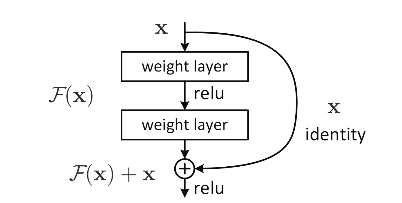 Residual learning: a building block.
The paper defines a residual block as \(y = F(x, W_i) + x\), where $F$ is the residual function learned by a few stacked layers, and the shortcut connection adds the input $x$ directly to the output of $F$ via element-wise addition; this design adds no extra parameters or computational cost.
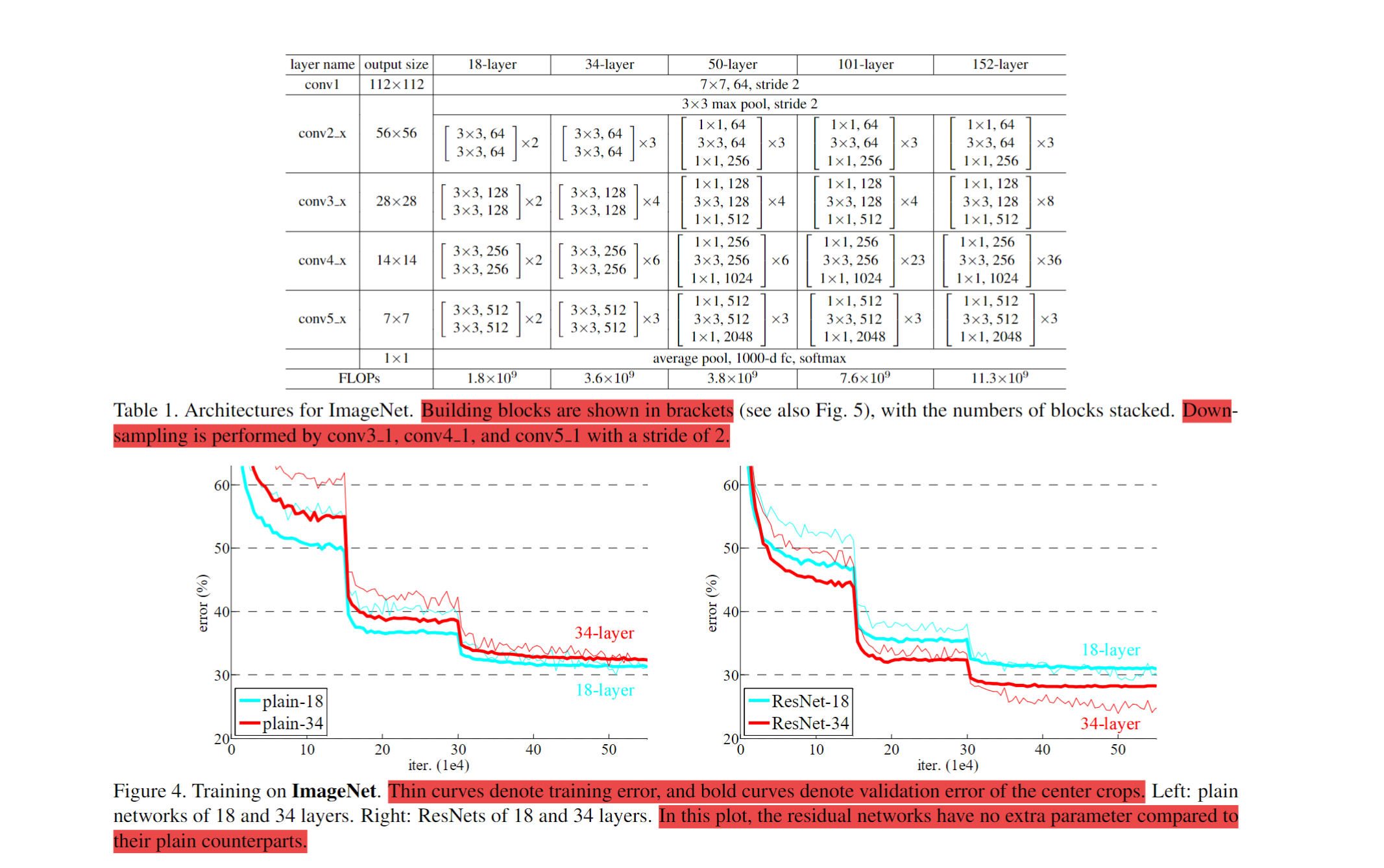
Their experiments on ImageNet and CIFAR-10 datasets showed that:
- ResNets are easy to optimize (converges faster), but the counterpart “plain” nets exhibit higher training error when the depth increases;
- ResNets can easily enjoy accuracy gains from greatly increased depth, producing results substantially better than previous networks.
Something to pay attention to!!!
To ensure compatibility in residual blocks, the input $x$ and residual output $F(x)$ must have matching dimensions; if not, a linear projection $W_s x$ is used via the shortcut. However, identity mappings are preferred for their simplicity and effectiveness. The residual function $F$ is flexible and typically composed of 2–3 layers (often convolutional), as single-layer $F$ offers no observed benefits.
- Identity vs. Projection Shortcuts: Three shortcut strategies were compared:
- Option A: Zero-padding for increasing dimensions; all shortcuts are parameter-free.
- Option B: Projection shortcuts for increasing dimensions; others are identity.
- Option C: All shortcuts are projection-based. Projection shortcuts offer only minor gains over identity shortcuts, making identity mappings the preferred choice for reducing complexity without sacrificing performance.
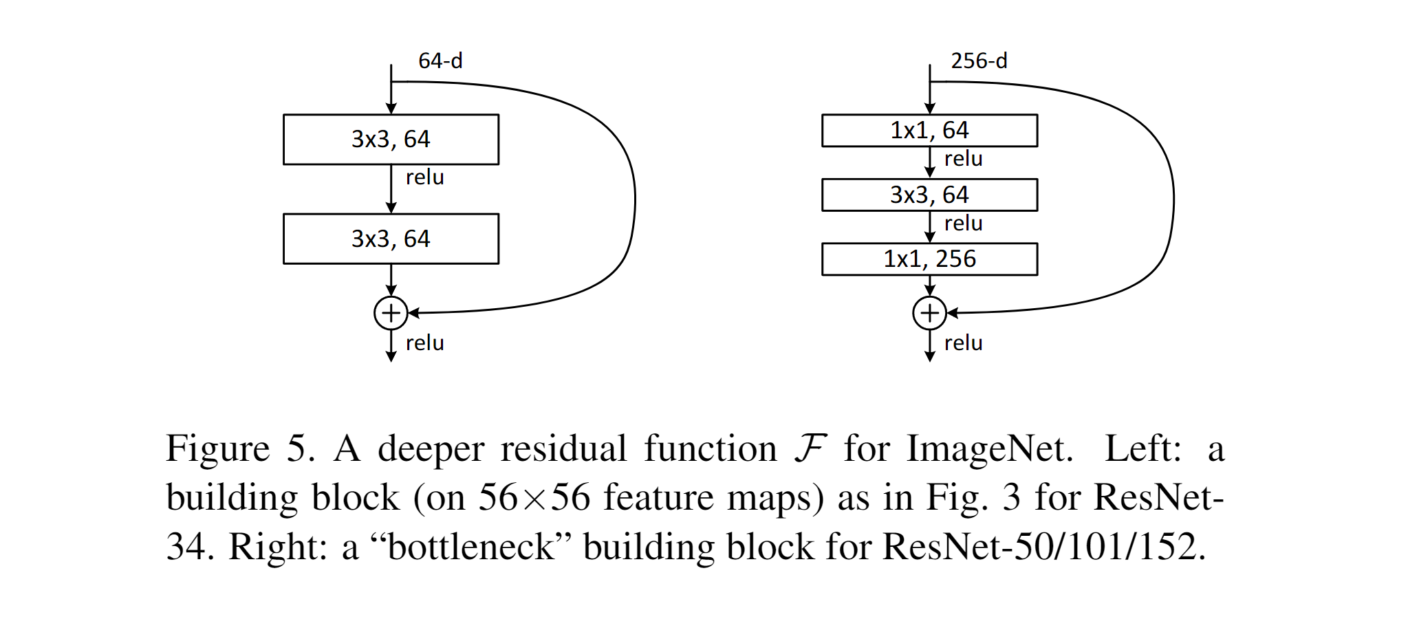
- Deeper Bottleneck Architectures: To reduce training time on ImageNet, a bottleneck block design is introduced. Each residual function F(x) consists of three layers:
1×1convolution (reduces dimensions),3×3convolution (core computation),1×1convolution (restores dimensions). If the shortcut uses a projection instead of identity, it doubles the model size and time complexity. Therefore, identity shortcuts are favored for efficiency, especially in bottleneck structures.
 Skip Connexion
Why it works?
The degradation problem suggests that the solvers might have difficulties in approximating identity mappings by multiple nonlinear layers. With the residual learning reformulation, if identity mappings are optimal, the solvers may simply drive the weights of the multiple nonlinear layers toward zero to approach identity mappings. In real cases, it is unlikely that identity mappings are optimal, but our reformulation may help to precondition the problem. If the optimal function is closer to an identity mapping than to a zero mapping, it should be easier for the solver to find the perturbations with reference to an identity mapping, than to learn the function as a new one.
Network Architectures & Implementation
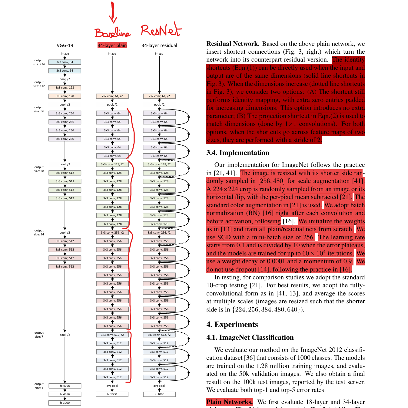
Residual networks are constructed by inserting shortcut connections into plain networks. Identity shortcuts are used when input and output dimensions are equal.
When dimensions differ (e.g., due to increased channels), two options are considered:
- Option A: Use identity mapping with zero-padding (no additional parameters).
- Option B: Use a projection shortcut via 1×1 convolutions to match dimensions (adds parameters). When shortcuts span feature maps of different sizes, they are applied with a stride of 2.
 Skip Connexion
Implementation Details (ImageNet):
- Data Augmentation:
- Shorter side of the image is randomly sampled in
[256, 480]. - A random
224×224crop is taken (or its horizontal flip). - Per-pixel mean subtraction and standard color augmentation are applied.
- Shorter side of the image is randomly sampled in
- Network Design:
- Batch Normalization (BN) is used after each convolution and before activation.
- No Dropout is used, following common practice.
- Training Setup:
- Optimizer: SGD with momentum
0.9. - Mini-batch size:
256. - Learning rate: starts at
0.1, divided by10on plateaus. - Total training: up to
60kiterations. - Weight decay:
0.0001. - All plain and residual networks are trained from scratch.
- Optimizer: SGD with momentum
 Skip Connexion
Common Misconceptions
- Degradation in deeper networks is not caused by overfitting.
- Batch Normalization prevents vanishing/exploding gradients, so degradation is not a gradient issue.
- The deeper networks’ training difficulty likely stems from slow convergence rather than signal degradation.
Ressources
- YouTube:
- Aladdin Persson: Pytorch ResNet implementation from Scratch
- Professor Bryce: Residual Networks and Skip Connections (DL 15)
Maciej Balawejder: [ResNet Paper Explained & PyTorch Implementation](https://youtu.be/wOuaGvxbtZo?si=hczOMHi88JhtHPVs) - Yannic Kilcher: [Classic] Deep Residual Learning for Image Recognition (Paper Explained)
- Priyam Mazumdar: Going Deeper with Residual Connections: ResNet Implementation
- Futher explorations:
An obstacle to answering this question was the notorious problem of vanishing/exploding gradients, which hamper convergence from the beginning. This problem, however, has been largely addressed by normalized initial ization and intermediate normalization layers, which enable networks with tens of layers to start converging for stochastic gradient descent (SGD) with backpropagation
Papers to explore: